Everything about SQL

This article will give all you wanted to know about databases and how to write queries we are going to see simple queries to some advance and complex queries. Now the main agenda of this article is to make you comfortable in writing complex queries. In the end, there will be some resources and practice sets where you can practice queries.

Before moving to the queries, we need to see some basic terminologies.

What is Database?

The database is an organized collection of structured data to make it easily accessible, manageable and update. In simple words, you can say, a database is a place where the data is stored. You can take the library as an example where, the library is the database and the books are the data. Books of different genres which are organized and stored in their respective section are what database is organizing and storing data.

What is Database Management System (DBMS)?

A Database Management System (DBMS) is software that is used to manage the Database. A DBMS basically serves as an interface between the database and its end-users or programs, allowing users to retrieve, update, and manage how the information is organized and optimized. A DBMS also facilitates oversight and control of databases, enabling a variety of administrative operations such as performance monitoring, tuning, and backup and recovery.

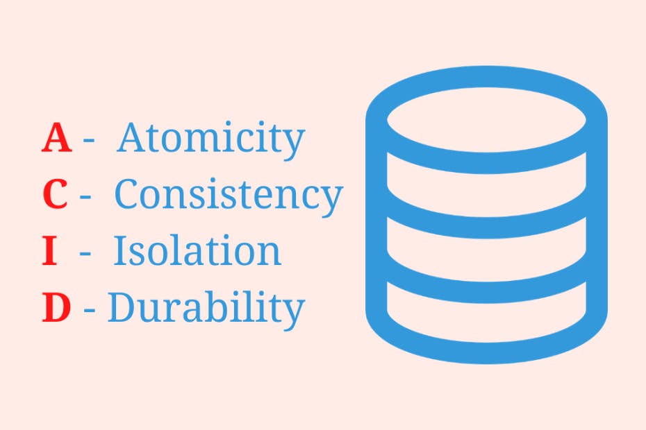
ACID properties

Atomicity

By this, we mean that either the entire transaction takes place at once or doesn’t happen at all. There is no midway i.e. transactions do not occur partially. Each transaction is considered as one unit and either runs to completion or is not executed at all. It involves the following two operations.

—Abort: If a transaction aborts, changes made to the database are not visible.
—Commit: If a transaction commits, changes made are visible. Atomicity is also known as the ‘All or nothing rule’.

Example:

Consider the following transaction T consisting of T1 and T2: Transfer of 100 from account X to account Y.

If the transaction fails after completion of T1 but before completion of T2. ( say, after write(X) but before write(Y)), then the amount has been deducted from X but not added to Y. This results in an inconsistent database state. Therefore, the transaction must be executed in its entirety in order to ensure the correctness of the database state.

Consistency

This means that integrity constraints must be maintained so that the database is consistent before and after the transaction. It refers to the correctness of a database. Referring to the example above, The total amount before and after the transaction must be maintained. Total before T occurs = 300 + 200 = 500. Total after T occurs = 400 + 100 = 500. Therefore, the database is consistent. Inconsistency occurs in case T1 completes but T2 fails. As a result, T is incomplete.

Isolation

This property ensures that multiple transactions can occur concurrently without leading to the inconsistency of the database state. Transactions occur independently without interference. Changes occurring in a particular transaction will not be visible to any other transaction until that particular change in that transaction is written to memory or has been committed. This property ensures that the execution of transactions concurrently will result in a state that is equivalent to a state achieved these were executed serially in some order.

Durability

This property ensures that once the transaction has completed execution, the updates and modifications to the database are stored in and written to disk and they persist even if a system failure occurs. These updates now become permanent and are stored in non-volatile memory. The effects of the transaction, thus, are never lost.

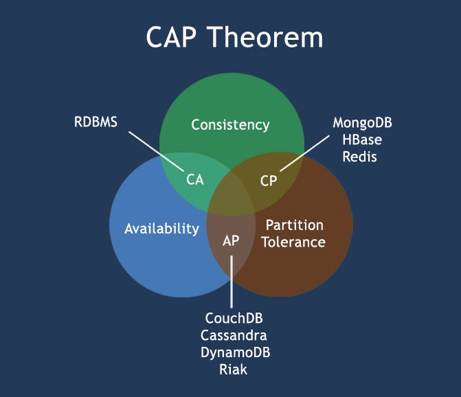
CAP theorem

The CAP theorem (also called Brewer’s theorem) states that a distributed database system can only guarantee two out of these three characteristics: Consistency, Availability, and Partition Tolerance.

Consistency

A system is said to be consistent if all nodes see the same data at the same time.

Simply, if we perform a read operation on a consistent system, it should return the value of the most recent write operation. This means that the read should cause all nodes to return the same data, i.e., the value of the most recent write.

Availability

Availability in a distributed system ensures that the system remains operational 100% of the time. Every request gets a (non-error) response regardless of the individual state of a node.

Partition Tolerance

This condition states that the system does not fail, regardless of if messages are dropped or delayed between nodes in a system.

Partition tolerance has become more of a necessity than an option in distributed systems. It is made possible by sufficiently replicating records across combinations of nodes and networks.

Normalization

Normalization is the process of minimizing redundancy from a relation or set of relations. Redundancy in relation may cause insertion, deletion and update anomalies. So, it helps to minimize the redundancy in relations. Normal forms are used to eliminate or reduce redundancy in database tables.

There are different types of Normal Forms to store the clean and well-structured data:

First normal form:

If a relation contains a composite or multi-valued attribute, it violates the first normal form or relation is in the first normal form if it does not contain any composite or multi-valued attribute. A relation is in first normal form if every attribute in that relation is singled valued attribute.

Eg:

ID   Name   Courses
------------------
1    A      c1, c2
2    B      c3
3    C      c2, c3

The above table "Courses" is a multi-valued attribute so it is not in 1NF.

To make it 1NF we need to make "Courses" in a single-valued attribute. The below table is in the 1NF.

ID   Name   Course
------------------
1    A       c1
1    A       c2
2    B       c3
3    C      c2
3    C       c3

Second normal form:

To be in second normal form, a relation must be in first normal form and relation must not contain any partial dependency. A relation is in 2NF if it has No Partial Dependency, i.e., no non-prime attribute (attributes which are not part of any candidate key) is dependent on any proper subset of any candidate key of the table.

Eg:

STUD_ID           COURSE_NO        COURSE_FEE
----------------------------------------------
1                     C1                  1000
2                     C2                  1500
1                     C4                  2000
4                     C3                  1000
4                     C1                  1000
2                     C5                  2000

Looking above example, it is 1NF cause all the value is single-valued attribute, but still, we cannot find COURSE_FEE with the help of STUD_ID so there is a partial dependency so it is not in 2NF.

Below is the example of 2NF.

       Table 1  

STUD_NO            COURSE_NO 
----------------------------- 
1                       C1                  
2                       C2                  
1                       C4                  
4                       C3                  
4                       C1      


        Table 2
COURSE_NO                COURSE_FEE  
-----------------------------------   
    C1                        1000
    C2                        1500
    C3                        1000
    C4                        2000
    C5                        2000

We split the data into 2 tables now, there is no partial dependency and the table is in 2NF.

Third normal form

A relation is in the third normal form if there is no transitive dependency for non-prime attributes as well as it is in the second normal form. A relation is in 3NF if at least one of the following conditions holds in every non-trivial function dependency X –> Y

X is a super key.
Y is a prime attribute.

Eg:

consider relation R(A, B, C, D, E) A -> BC, CD -> E, B -> D, E -> A

All possible candidate keys in the above relation are {A, E, CD, BC} All attributes are on the right sides of all functional dependencies are prime.

Indexes

Indexing is a way to optimize the performance of a database by minimizing the number of disk accesses required when a query is processed. It is a data structure technique that is used to quickly locate and access the data in a database.

Indexes are created using a few database columns.

The first column is the Search key that contains a copy of the primary key or candidate key of the table. These values are stored in sorted order so that the corresponding data can be accessed quickly.
The second column is the Data Reference or Pointer which contains a set of pointers holding the address of the disk block where that particular key value can be found.

Transactions

A transaction can be defined as a group of tasks. A single task is the minimum processing unit that cannot be divided further.

Let’s take an example of a simple transaction. Suppose a bank employee transfers Rs 500 from A's account to B's account. This very simple and small transaction involves several low-level tasks.

The below code block shows all the level transaction happen when someone sends money from one bank to another bank.

A's account

Open_Account(A)
Old_Balance = A.balance
New_Balance = Old_Balance - 500
A.balance = New_Balance
Close_Account(A)

B's account

Open_Account(B)
Old_Balance = B.balance
New_Balance = Old_Balance + 500
B.balance = New_Balance
Close_Account(B)

Locking Mechanism

The locking mechanism is one of the means of concurrency control. Whenever multiple transactions are made a lock on data is needed. Therefore we require a mechanism to lock the requests and prevent the database from going to an inconsistent state. In this, the lock manager and the transactions exchange messages to lock and unlock the data items. The locking protocol requires a data Structure to implement it, and therefore the best data structure is the LOCK TABLE.

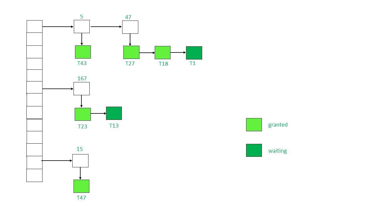
The transactions that are requesting a lock are having a downward arrow below them. Therefore we can see the locked data items are 5,47,167, 15. The colour of the node represents the status i.e. granted or waiting.

In the beginning, the lock table is empty and none of the data items is locked.

Then when the lock manager receives a request to lock the particular data item from a Transaction for instance T(i) on data item P(i): then 2 cases might appear

P(i) is already granted a lock, then a new node will be added to the end of the linked list which contains the information about the kind of request made.
P(i) is not already locked, a linked list will be created and the lock will be granted.

Now if the requested lock mode is compatible with the current transaction lock mode then T(i) will acquire the lock too and the status will be “Granted” else “ Waiting”.

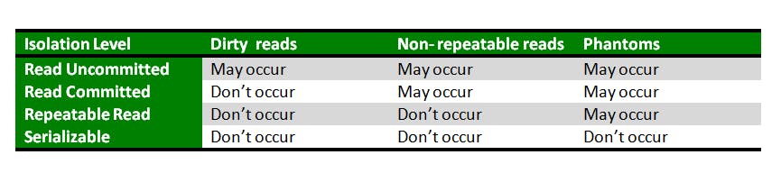
Isolation levels

Isolation levels define the degree to which a transaction must be isolated from the data modifications made by any other transaction in the database system.

The SQL standard defines four isolation levels:

Read Uncommitted: Read Uncommitted is the lowest isolation level. At this level, one transaction may read not yet committed changes made by other transactions, thereby allowing dirty reads. At this level, transactions are not isolated from each other.
Read Committed: This isolation level guarantees that any data read is committed at the moment it is read. Thus it does not allows dirty read. The transaction holds a read or write lock on the current row, and thus prevent other transactions from reading, updating or deleting it.
Repeatable Read: This is the most restrictive isolation level. The transaction holds read locks on all rows it references and writes locks on all rows it inserts, updates, or deletes. Since other transaction cannot read, update or delete these rows, consequently, it avoids non-repeatable read.
Serializable: This is the highest isolation level. A serializable execution is guaranteed to be serializable. Serializable execution is defined to be an execution of operations in which concurrently executing transactions appears to be serially executing.

What is a structured query language (SQL)?

Structured Query language SQL is pronounced as “S-Q-L” or sometimes as “See-Quel” which is the standard language for dealing with Relational Databases.

It is effectively used to insert, search, update, delete, modify database records. It doesn’t mean SQL cannot do things beyond that. In fact, it can do a lot more other things as well. SQL is regularly used not only by database administrators but also by the developers to write data integration scripts and data analysts.

Now that you guys have understood what SQL is. We can start working on Queries.

I am going to use PostgreSQL, hope you have installed it. If not, set up PostgreSQL using below links.

Dataset

We are going to use the dataset from pg exercises. It's a perfect dataset for practising simple queries to complex queries.

Download dataset

Start the psql server

~ psql

Create database named exercises, where we are going to load our dataset.

your_name=# create database exercises;
your_name=# \q

~ psql exercises < "path-to-your-downloaded-data"

Dataset is loaded and ready to work on.

Queries

Now, If you are reading this, means you have set up the PostgreSQL and also loaded the .sql data in your system.

We are going to use a terminal for writing Queries.

Open psql server in terminal

~ psql

List the databases

your_name=# \l
                                  List of databases
   Name    |  Owner   | Encoding |   Collate   |    Ctype    |   Access privileges
-----------+----------+----------+-------------+-------------+--------
 exercises | your_name | UTF8     | en_US.UTF-8 | en_US.UTF-8 |

You can see, exercises database is there we just have to switch to that database, then we can access the tables.

Switch databases

\c exercises
exercises=# \dn

  List of schemas
  Name  |  Owner
--------+----------
 cd     | your_name
 public | Postgres

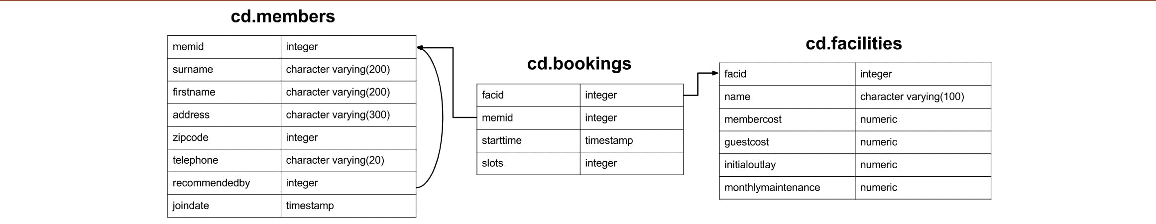
Now here cd is a schema, and the below image shows the structure of the table and their relations.

Screenshot 2021-08-23 at 9.28.00 PM.png

Now, we can practice some of the basic Queries

SELECT statement

The SELECT statement is used to select data from a database.

select particular column

> select telephone from cd.members
  limit 10;

    telephone
----------------
  (000) 000-0000
  555-555-5555
  555-555-5555
  (844) 693-0723
  (833) 942-4710
  (844) 078-4130
  (822) 354-9973
  (833) 776-4001
  (811) 433-2547
  (833) 160-3900
(10 rows)

Here, the SELECT statement is used to retrieve the particular data or column from a table. above statement also has LIMIT which specifies the number of rows to be shown, it is used when there is a large dataset.

Select multiple columns

> select first name, surname from cd. members
  limit 10;

  first name | surname
  -----------+----------
  GUEST     | GUEST
  Darren    | Smith
  Tracy     | Smith
  Tim       | Rowman
  Janice    | Joplette
  Gerald    | Butters
  Burton    | Tracy
  Nancy     | Dare
  Tim       | Boothe
  Ponder    | Stibbons
(10 rows)

We can use specify multiple columns separated by ',' for selecting multiple columns.

Select all columns

> select * from cd.bookings
  limit 10;

   bookid | facid | memid |      starttime      | slots
--------+-------+-------+---------------------+-------
      0 |     3 |     1 | 2012-07-03 11:00:00 |     2
      1 |     4 |     1 | 2012-07-03 08:00:00 |     2
      2 |     6 |     0 | 2012-07-03 18:00:00 |     2
      3 |     7 |     1 | 2012-07-03 19:00:00 |     2
      4 |     8 |     1 | 2012-07-03 10:00:00 |     1
      5 |     8 |     1 | 2012-07-03 15:00:00 |     1
      6 |     0 |     2 | 2012-07-04 09:00:00 |     3
      7 |     0 |     2 | 2012-07-04 15:00:00 |     3
      8 |     4 |     3 | 2012-07-04 13:30:00 |     2
      9 |     4 |     0 | 2012-07-04 15:00:00 |     2
(10 rows)

We can use "*" for selecting all the data from a particular table.

WHERE clause

WHERE clause is applied to each row of data by checking specific column values to determine whether it should be included in the results or not.

Example of where clause

> select * from cd.facilities
  where monthlymaintenance < 50;

  facid |     name      | membercost | guestcost | initialoutlay | monthlymaintenance
  -------+---------------+------------+-----------+---------------+--------------------
      3 | Table Tennis  |          0 |         5 |           320 |                 10
      7 | Snooker Table |          0 |         5 |           450 |                 15
      8 | Pool Table    |          0 |         5 |           400 |                 15

As you can see all the entries with monthlymaintenance less than 50 is retrieved.

We can use logical operators like AND and OR for multiple conditions

> select * from cd.facilities
  where membercost > 0 and
  initialoutlay > 1000;

 facid |      name      | membercost | guestcost | initialoutlay | monthlymaintenance
-------+----------------+------------+-----------+---------------+--------------------
     0 | Tennis Court 1 |          5 |        25 |         10000 |                200
     1 | Tennis Court 2 |          5 |        25 |          8000 |                200
     4 | Massage Room 1 |         35 |        80 |          4000 |               3000
     5 | Massage Room 2 |         35 |        80 |          4000 |               3000
     6 | Squash Court   |        3.5 |      17.5 |          5000 |                 80

BETWEEN / NOT BETWEEN

As the name defines it is widely used for extracting data in range.

> select * from cd.bookings
  where bookid between 3 and 5;

  bookid | facid | memid |      starttime      | slots
--------+-------+-------+---------------------+-------
      3 |     7 |     1 | 2012-07-03 19:00:00 |     2
      4 |     8 |     1 | 2012-07-03 10:00:00 |     1
      5 |     8 |     1 | 2012-07-03 15:00:00 |     1

Here we get the column from range 3 and 5 of bookid. Similarly we can use NOT BETWEEN.

> select * from cd.bookings
  where bookid not between 3 and 5;
  limit 10;


   bookid | facid | memid |      starttime      | slots
--------+-------+-------+---------------------+-------
      0 |     3 |     1 | 2012-07-03 11:00:00 |     2
      1 |     4 |     1 | 2012-07-03 08:00:00 |     2
      2 |     6 |     0 | 2012-07-03 18:00:00 |     2
      6 |     0 |     2 | 2012-07-04 09:00:00 |     3
      7 |     0 |     2 | 2012-07-04 15:00:00 |     3
      8 |     4 |     3 | 2012-07-04 13:30:00 |     2
      9 |     4 |     0 | 2012-07-04 15:00:00 |     2
     10 |     4 |     0 | 2012-07-04 17:30:00 |     2
     11 |     6 |     0 | 2012-07-04 12:30:00 |     2
     12 |     6 |     0 | 2012-07-04 14:00:00 |     2

IN/ NOT IN

As named, it is used to get data if it is present in some list or according to the user conditions

> select * from cd.bookings
  where bookid in (1,2,15,5);

   bookid | facid | memid |      starttime      | slots
--------+-------+-------+---------------------+-------
      1 |     4 |     1 | 2012-07-03 08:00:00 |     2
      2 |     6 |     0 | 2012-07-03 18:00:00 |     2
      5 |     8 |     1 | 2012-07-03 15:00:00 |     1

the above Query listed all the entries if the book id is in that list.

Similarly, we can do it for NOT IN.

> select * from cd.bookings
  where bookid not in (1,2,15,5,7,9,10)
  limit 10;

   bookid | facid | memid |      starttime      | slots
--------+-------+-------+---------------------+-------
      0 |     3 |     1 | 2012-07-03 11:00:00 |     2
      3 |     7 |     1 | 2012-07-03 19:00:00 |     2
      4 |     8 |     1 | 2012-07-03 10:00:00 |     1
      6 |     0 |     2 | 2012-07-04 09:00:00 |     3
      8 |     4 |     3 | 2012-07-04 13:30:00 |     2
     11 |     6 |     0 | 2012-07-04 12:30:00 |     2
     12 |     6 |     0 | 2012-07-04 14:00:00 |     2
     13 |     6 |     1 | 2012-07-04 15:30:00 |     2
     14 |     7 |     2 | 2012-07-04 14:00:00 |     2
     16 |     8 |     3 | 2012-07-04 18:00:00 |     1

LIKE operator

LIKE operator is used to perform conditions on the strings. "%" operators is for multiple and " _ " operators is for one.

> select firstname from cd.members
  where firstname like 'T%';

   firstname
  -----------
    Tracy
    Tim
    Tim
    Timothy

Here, in the above example I received the firstname which starts from "T", "%% operator is used so that multiple characters can come after "T". this we can perform operations on strings

Sorting (order by)

ORDER BY is used to order the column in ascending or descending, by default it's ascending or you can use 'asc' or 'desc' for ascending and descending similarly.

> select firstname, surname from cd.members
  order by firstname desc
  limit 10;

   firstname | surname
  -----------+----------
    Tracy     | Smith
    Timothy   | Baker
    Tim       | Boothe
    Tim       | Rownam
    Ramnaresh | Sarwin
    Ponder    | Stibbons
    Nancy     | Dare
    Millicent | Purview
    Matthew   | Genting
    John      | Hunt

Here the name has been sorted descending and the top 10 entries are retrieved using the "LIMIT" keyword.

We can also use the "OFFSET" keyword to get the limited data.

Get the data of id from 3 to 5 using offset

> select memid,firstname, surname from cd.members
  limit 3 offset 3;

   memid | firstname | surname
-------+-----------+----------
     3 | Tim       | Rownam
     4 | Janice    | Joplette
     5 | Gerald    | Butters

Offset allows to start from that number and limit helps to get the particular number of rows.

JOINS

A JOIN clause is used to combine rows from two or more tables, based on a related column between them.

Inner JOIN

Inner join helps to combine the 2 tables. it will return if there is a proper match. it won't return the column with null values by default JOIN clause is Inner join

> select bks.facid, fac.name, bks.slots from cd.bookings bks 
  join cd.facilities fac on bks.facid = fac.facid
  limit 10;

  facid |      name      | slots
-------+----------------+-------
    0 | Tennis Court 1 |     3
    0 | Tennis Court 1 |     3
    0 | Tennis Court 1 |     3
    0 | Tennis Court 1 |     3
    0 | Tennis Court 1 |     3
    0 | Tennis Court 1 |     3
    0 | Tennis Court 1 |     3
    0 | Tennis Court 1 |     3
    0 | Tennis Court 1 |     3
    0 | Tennis Court 1 |     3

In above example, 'bks' and 'fac' is the alias given to the table so that it gets easy to recognize which table's the column we are trying to access and we inner join the two tables on the facid.

LEFT JOIN

Returns all rows from the left table, even if there are no matches in the right table.
RIGHT JOIN

Returns all rows from the right table, even if there are no matches in the left table.
FULL JOIN

It combines the results of both left and right outer joins.

The joined table will contain all records from both the tables and fill in NULLs for missing matches on either side.

unfortunately, we don't have such conditions to show that in practice but below is the link you can visualize that is how joins work in SQL.

Learn JOINS from here

Expressions

We can use expressions like multiplication and calculations while selecting the column and renamed it and create another column.

> select name, membercost+guestcost as total_cost from cd.facilities
  limit 10;

        name       | total_cost
  -----------------+------------
    Tennis Court 1  |         30
    Tennis Court 2  |         30
    Badminton Court |       15.5
    Table Tennis    |          5
    Massage Room 1  |        115
    Massage Room 2  |        115
    Squash Court    |       21.0
    Snooker Table   |          5
    Pool Table      |          5

So, in the above example, we added the membercost and guestcost and created a new column as total_cost using "AS" for naming and limit the first 10 entries. This is how we can perform multiple expressions and output the data.

Aggregations

In addition to the simple expressions, SQL also supports the use of aggregate expressions (or functions) that allow you to summarize information about a group of rows of data.

Some common aggregate functions are, Count, Sum, Min, Max which makes our work fast and effective.

> select count(*) from cd.facilities;

   count
  -------
      9
(1 row)

The above example shows, how many facilities exist - simply produce a total count.

> select facid, sum(slots) as "Total Slots"
    from cd.bookings
    where
        starttime >= '2012-09-01'
        and starttime < '2012-10-01'
    group by facid
  order by sum(slots);  


   facid | Total Slots
  -------+-------------
      5 |         122
      3 |         422
      7 |         426
      8 |         471
      6 |         540
      2 |         570
      1 |         588
      0 |         591
      4 |         648

The above example, gives the total number of slots booked per facility in the the month of September 2012 and sorted by the number of slots.

GROUP BY / HAVING

It is used with the aggregate functions, it groups rows that have the same values into summary rows, like "find the number of customers in each country".

"GROUP BY" clause comes after the "WHERE" clause so to filter the "GROUP BY" data luckily we have the "HAVING" clause.

We will see this thing in action.

Suppose we need to produce a list of facilities with more than 1000 slots. we can get the results with the help of group by and having.

> select facid, sum(slots) as "Total Slots"
    from cd.bookings
    group by facid
    having sum(slots) > 1000
    order by facid;  


     facid | Total Slots
    -------+-------------
        0 |        1320
        1 |        1278
        2 |        1209
        4 |        1404
        6 |        1104

in the above example, we used aggregate function SUM to get total the slots then we group by with "facid" which grouped the results with the distinct facid and we used having clause to filter out the entries whose slots is greater than 1000.

Subqueries

Subqueries is like the nested Queries like we have a query inside a query

A simple example is, suppose if you want to create a new table with your result query we can simply do it by using Subqueries.

>create table subquery as (
    select distinct facid, name from cd.facilities
    order by facid
);

SELECT 9

To check the output write the below command.

> \dt

          List of relations
 Schema |   Name   | Type  |  Owner
--------+----------+-------+----------
 public | subquery | table | your_name

> select * from subquery;

 facid |      name
-------+-----------------
     0 | Tennis Court 1
     1 | Tennis Court 2
     2 | Badminton Court
     3 | Table Tennis
     4 | Massage Room 1
     5 | Massage Room 2
     6 | Squash Court
     7 | Snooker Table
     8 | Pool Table
(9 rows)

Now, almost every basic to some advanced concept is covered. but we were working on a particular dataset. what if we need to create our own tables and put the entries inside it and perform Queries on that table.

Triggers

Triggers are the SQL statements that are automatically executed when there is any change in the database. The triggers are executed in response to certain events(INSERT, UPDATE or DELETE) in a particular table. These triggers help in maintaining the integrity of the data by changing the data of the database in a systematic fashion.

one real-life example, If you sign up for a new website, then you get a welcome mail from that site one possibility is that triggers are used that Whenever a new user sign up then the system should send the welcome mail to the new user.

let's see trigger in practice.

> create table student (
    id bigint,
    name varchar(50),
    choclates varchar(50)
);

> insert into student values (1,'Vivek',10),
    (2,'Ronaldo',5),
    (3,'Messi',2),
    (4,'lewandowski',6);

> select * from student;

 id |    name     | chocolates
----+-------------+-----------
  1 | Vivek       | 10
  2 | Ronaldo     | 5
  3 | Messi       | 2
  4 | lewandowski | 6
(4 rows)

As you can see, I created a dummy table of students to demonstrate how the trigger works.

now there are 3 columns of id, name, chocolates what if I want to create a trigger that will add 10 chocolates to every student Whenever a new student is inserted in the table

lets see,

> create trigger add_choclates
    before
    insert
    on student
    for each row
    set choclates = choclates+10;

> insert into student values (5,'Neymar',5);

> select * from student;
 id |    name     | choclates
----+-------------+-----------
  1 | Vivek       | 20
  2 | Ronaldo     | 15
  3 | Messi       | 12
  4 | lewandowski | 16
  5 | Neymar      | 15
(5 rows)

Here, we can see that the data is updated and 10 chocolates are added to every row with the help of a trigger.

CRUD (create, read, update, delete)

CREATE

We are going to create a simple table and perform all the above operations and at the end we will drop the table.

> create table test (
    id bigint,
    name varchar(50),
    phone_number varchar(20)
  );

  CREATE TABLE

To check if the table is created use \dt

> \dt

          List of relations
 Schema |   Name   | Type  |  Owner
--------+----------+-------+----------
 public | subquery | table | vivekcr7
 public | test     | table | vivekcr7

As we can see the test table is created. now we going to insert the data in it.

INSERT

Now, we will insert values into our newly created table.

> insert into test values(1,'vivek','+91 1234567890');

  INSERT 0 1

Quickly write a select query to check if data is inserted or not.

> select * from test;

   id | name  |  phone_number
  ----+-------+----------------
    1 | vivek | +91 1234567890
(1 row)

As we can see data is updated what if we want to insert multiple data at once

> insert into test values(2,'ronaldo','+91 2345678987'),
    (3,'messi','+91 45678734567'),
    (4,'lewandowski','+91 9876567434'),
    (5,'neymar','+91 984524562');

    INSERT 0 4

> select * from test;

     id |    name     |  phone_number
    ----+-------------+-----------------
        1 | vivek       | +91 1234567890
        2 | ronaldo     | +91 2345678987
        3 | messi       | +91 45678734567
        4 | lewandowski | +91 9876567434
        5 | neymar      | +91 984524562
(5 rows)

UPDATE

Now, the update is basically used if we put some wrong entries.

Like what if the entry with id 3 name is wrong. so to change that we have to use the "UPDATE" clause.

> update test
  set name = 'Dybala'
  where id = 3


> select * from test
    order by id;

     id |    name     |  phone_number
    ----+-------------+-----------------
        1 | vivek       | +91 1234567890
        2 | ronaldo     | +91 2345678987
        3 | Dybala      | +91 45678734567
        4 | lewandowski | +91 9876567434
        5 | neymar      | +91 984524562
(5 rows)

As you can see the name has changed from 'messi' to 'Dybala' using the update clause.

DELETE / DROP

Now we have come to our last topic, which is the delete and drop statement.

Delete row with id 4.

> delete from test
    where id = 4;

    DELETE 1

> select * from test
    order by id;

 id |  name   |  phone_number
----+---------+-----------------
  1 | vivek   | +91 1234567890
  2 | ronaldo | +91 2345678987
  3 | Dybala  | +91 45678734567
  5 | neymar  | +91 984524562
(4 rows)

Now row with id 4 is deleted what if you want to delete all the entries.

> delete from test;

  DELETE 4

> select * from test;

     id | name | phone_number
    ----+------+--------------
    (0 rows)

Now all the rows have been deleted. now drop the table using the "DROP" statement.

> drop table test;

  DROP TABLE

> \dt

            List of relations
 Schema |   Name   | Type  |  Owner
--------+----------+-------+----------
 public | subquery | table | vivekcr7
(1 row)

Now the table is also deleted. now we also going to drop our database exercises.

For that first move to a different database using '\c', cause we cannot drop an active database.

> \c postgres

> drop database exercises;

    DROP DATABASE

Now the database is deleted to check to write the below command

> \l

it will give you the list of databases.

References

Conclusion

Hope you have understood all the concepts, Database is a very vast topic I have tried to cover the important ones which every developer should know. Above is the 2 reference links will be more helpful if you refer and practice queries from there.

Thank you for staying till the end of the article.

Author

@Vivek Dubey

Vivek Dubey's Blog